Scores and Quality Ranking

At its heart, reviewer scoring is simply a way to rank the relative quality of all the products a given reviewer has sampled. Typically, a higher score indicates a higher quality sample. But the actual scale range can be completely arbitrary for each reviewer, including the number of gradations between individual scores.

And that is fine – as long as you are only planning to compare scores within one reviewer’s catalog, and not across multiple reviewers. Typically, you could only compare across reviewers if you knew they were making an explicit attempt the match their scoring (i.e., a group of reviewers aligned with one particular site).

In real life however, it is unlikely that any one reviewer (or closely aligned group) is going to try everything you are potentially interested in. And when it comes to matters of personal taste, no one reviewer is going to be entirely consistent (given the subjective nature of experience), nor are they likely to necessarily be a good match to your personal preferences. Add to that the fact that the topic in question here – whiskies – are subject to significant individual batch variation, and it gets increasingly difficult to find a consistent way to make sense of overall whisky quality from disparate sources.

What I am going to do over these various Methodology pages is explain how you can break down all the sources of variation, and re-combine them in a way that provides a scientifically-valid (that is to say, a statistically-valid) method of integrating reviewer scores.  I call this the Meta-Critic Score on this site.

How Variable are Reviewers?

To get started, we are somewhat lucky here – in practice, it seems like most whisky reviewers (and reviewers of liquor in general) try to follow a comparable rating system to that developed by Robert Parker for scoring wines. That is to say, they use a scoring range of 50-100 – with anything below 60 being deemed unacceptable for consumption.

But how consistent are they really?  I will discuss this further on my Review Biases and Limitations page. But for now lets start by exploring some some very basic descriptive statistics of individual reviewers.

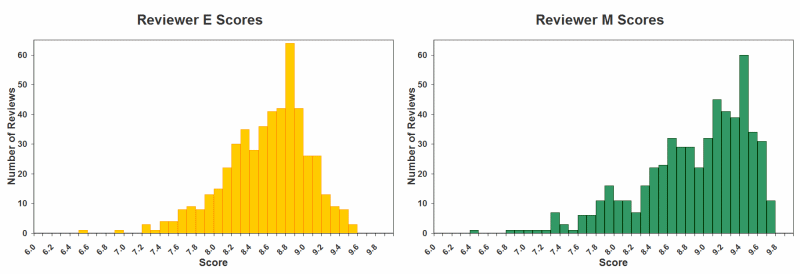
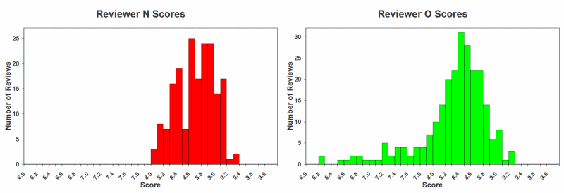
Below are frequency distributions showing how often individual scores are given by a handful of the expert reviewers tracked in my database. I am using the same anonymized reviewer coding as on my Review Biases and Limitations page. Note that these are the reviewer raw scores – they have not be corrected or adjusted in any way, except to be plotted on a consistent x-axis score range (presented as base 10). The y-axis refers to the actual number of whiskies in my database that have received that particular score.

It seems pretty clear from the above that there is a lot variability in how individual reviewers choose to interpret the score range. Note that the specific whiskies each reviewer has chosen to review are different as well, which is a further confounding factor at this stage.

Given this apparent variability, you cannot simply go ahead and average the raw scores.  Imagine what would happen if you combined reviewer C and O for example, or M and N. Because of how differently each apparently applies their scoring range, you would get a very misleading result.

By the way, a funny thing happens if you try do try combine all the skewed reviewer scores together, across each of the individual whiskies in my dataset:

I add the “X” above, because this is the wrong way to do things. But it produces an interesting result that is likely to fool the casual observer into thinking it is valid.

If you look at all the individual reviewer distributions above, you will see that they all are somewhat skewed (i.e., none have the perfectly smooth and symmetrical bell-shaped “normal” distribution you may have hoped for). But since they are using different parts of the scale range, when you lump them all together you get something that approximates the classic normal distribution (albeit one with a slightly extended left tail).

Again, this simple averaging of the raw scores produces a spurious finding that will NOT help you understand the true ranking of the whiskies across reviewers. You need to take into account the specific whiskies they review, as well as how they apply the scoring system.

Assumption of Normality

Something everyone learns early in introductory statistics is that many statistical tests (particularly parametric ones) have an underlying assumption of normality. They are thus very sensitive to any deviations from the normal probability distribution, as these can produce spurious “positive” results (that are in fact nothing more than an artifact of the analysis method churning away on something that doesn’t match its requirements). Most people then go on to promptly ignore this fact, since it complicates their life (and they often can’t directly test for it anyway). 😉

But in our case, we already have a very strong inkling from the handful of individual distributions above that normality is a bit skewed in our dataset.

Indeed, this is a fundamental design problem that anyone who works with scoring systems quickly discovers. By its literal description, the Parker wine scoring scheme (ostensibly adopted by most liquor reviewers) is supposed to be normally distributed. In this classic 50-100 scoring system, 75 is defined as an average product (and the literal average expected score).

But as you can see above, none of the reviewers really fit that pattern (although some are closer to it than others).  Instead, what happens over time is that “grade inflation” invariably winds up compressing scores at the high-end (right-side of the graphs above), and stretching out scores at the low end (left side). The end result is that the “average” score is quite a bit higher for each reviewer than the numerical middle.  Indeed, if you look at all the raw scores on a per-reviewer basis, the average winds up being around ~85%.

While you may be getting discouraged at this point, buck up – we can actually overcome these problems fairly easily. 🙂

Is Being Skewed a Problem?

As it turns out, deviation from normality in reviewer scoring is not a problem for an integrative analysis. What matters here is whether or not reviewers are consistent in how they apply their scores. In other words, so long as they are skewed in a similar way, we can still adjust and combine their relative ranking results.

I’ll will work through the method over the coming methodology pages, but let me jump right to the conclusion – here is how a frequency distribution of the properly normalized Meta-Critic Scores looks, across all whiskies in my dataset (currently over 6600 data points, but rounded to nearest whole review number):

The graph above reflects what the combined Meta-Critic core distribution actually looks like, when properly integrating all reviewer scoring patterns. As you can probably tell, it does kind of look like an “average” of all those earlier individual distributions, adjusted for a common score range.

Integrating Reviewer Scores

I will get into creating the Meta-Critic Score in more detail on the subsequent Methodology pages. But the key take-home message here is that while the score distributions of each of the reviewers may look different, all show a fairly consistent pattern overall (and one that is represented in the final Meta-Critic Score). Specifically, while they typically approximate normality, they are consistently asymmetrical in the same way – namely, they all skew to the left (known as negative skewness).

The degree of skewness can actually be quantified, although this is trickier to interpret than you might think (i.e., there are many ways in which the distribution can be skewed either left or right).  For example, in the composite Meta-Critic summary above, you can see that in addition to a longer left tail (i.e., the bottom of the y-axis), the left “shoulder” is quite a bit wider as well (i.e., the upper part of the y-axis, nearing the apex). This is commonly the case for most reviewers – but not all. For example, look at Reviewer O at the top of the page – the distribution there is heavily skewed left at the tail, but actually has a lower “dropped” left shoulder.

If necessary, you can adjust distributions to correct for excessive skewness by a power transform (e.g., squaring or cubing to reduce negative skewness, square/cube-rooting for positive skewness). In general though, this is something you should avoid if you can.

For the Mata-Critic analysis, I follow a standard statistical rule-of-thumb to only adjust skewed reviewer data if the degree of skewness exceeds the typical average reviewer skewness by a factor of more than two standard deviation units. And then, I apply only as much of a transform as is necessary to bring the overall distribution to within those boundaries. For the 27 final reviewer groups that I currently track (as of February 2016), only one has needed this power transform (i.e., Reviewer O above).

I know I’m getting into the weeds a little here, but the point is that the underlying data has to be carefully examined to see if your analysis methods are valid, and that you are not failing any core assumptions or requirements. I continually measure and quantify the characteristics of my reviewer datasets, and make any adjustments as necessary to the analysis method.

Independence of Measures

Since I’m drifting off-topic a little, I thought I’d end this part of the methodology section with one of my little statistical peccadilloes. Namely, it’s important to remember that while consistently skewed distributions are not necessarily a problem when it comes to integrating scores, they are a problem when looking at some other distribution characteristics more generally.

In particular, the related concept of kurtosis, which most people use as a way to describe how “pointy” or “flat” a normal distribution is (i.e., the range of up-down variation in the curve).  What people often forget is that any method for calculating kurtosis is highly dependent on skewness (i.e., this is one case where deviations from normality really matter). In particular, asymmetrical “shoulders” in the distribution will produce significant excess kurtosis regardless of the overall “pointiness” of the distribution. So if you are finding a significant skewness in your data, don’t bother trying to measure kurtosis – it will likely mislead more than illuminate.

In the language of statistics, the skewness and kurtosis of a probability distribution are not independent. 🙂  To learn more, here’s a good old open-source article on their inter-relationship.

At this point, please see my Review Biases and Limitations page to further understand how the Meta-Critic Score is constructed.